Below you will find all the answers to the questions about climate you were afraid to ask……
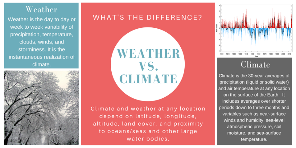
Weather vs Climate, What is the Difference?
Weather, Climate, and People: What are the Short- and Long-Term Impacts?
Weather and climate influence our lives daily. Whether it’s deciding to bring a jacket and umbrella on a walk or causing life-threatening issues like food insecurity and conflict abroad, these phenomena have both short- and long-term impacts.
Weather impacts people via temperature, windiness, rain, snow, ice, storminess, cloudiness, and air quality. It influences people’s decisions in clothing, transportation, and travel. Businesses and outdoor activities such as construction and repairs, landscaping and watering, sports and recreation, and meetings can change due to weather events. Even though some weather phenomena such as rain, wind, and storm might be relatively short, their impacts on a community or region may last for months or years depending on the severity of the event.
Though similar, the impacts of climate events last much longer than those of weather events, with some lasting for a few months, a few years or even a few decades. Climate events can damage or benefit supply and demand for food, water, and electricity. Therefore, the health of people, animals, and marine and land ecosystems rely on accessibility to such resources. Climate events can also impact river flows and, consequently, transportation and commerce on waterways. In the last 1,000 years, climate events, especially droughts, which last from a few years to a few decades, can cause famines, water shortages, socio-economic and political instabilities, and political revolutions and armed conflicts within and among countries.
What are the Societal Consequences of Drought?
Epochs of North American Decadal Hydrologic Cycles and Their Societal Consequences
| Years (CE) | Epoch | Name | Societal Consequences |
|---|---|---|---|
| 1273 - 1298 | Dry | The Puebloan drought | Rapid declines and migrations of populations of the Anasazi, the Fremont, and the Lovelock cultures in the Western U.S.; and the Cahokian culture in the Mississippi River valley (Benson et al., 2007; Axtell et al., 2002) |
| 1299 - 1336 | Wet | - | - |
| 1346 - 1355 | Dry | Mississippian drought | Decline of complex societies in the Mississippi River valley, partly due to widespread, poor crop harvests and limited food storage facilities (Anderson et al., 1995; Milner, 1998). |
| 1378 - 1388 | Wet/Dry | Mississippian drought | Wet in the West, dry in the Mississippi River valley; further decline of societies in the Mississippi River valley |
| 1449 - 1458 | Dry | Mississippian drought | Severe drought in the Mississippi River valley and southern Plains; abandonment of Mississippian settlements in eastern Oklahoma and the area around the confluence of the Ohio and Mississippi Rivers (Thomas, 2000; Cobb and Butler, 2002) |
| 1563 - 1573 | Wet/Dry | Mississippian drought | Wet in the West, dry in the Mississippi River valley and the Northeast; |
| 1666 - 1674 | Dry | The Puebloan drought | Disease, deaths, and village abandonment due to famine (Sauer, 1980) |
| 1806 - 1808 | Dry | The Great American Desert | Reports of the Great Plains as a desert by the Zebulon Pike expedition (Wishart, 2004; Rosenberg, 2007) |
| 1810 - 1820 | Wet | - | Westward migration of people from the eastern U.S. tripled Missouri’s population in this epoch, demands for statehood for Missouri |
| 1820 - 1826 | Dry | The Great American Desert | Reports of the areas along the Missouri and Platte Rivers as a desert by the Stephen Long expedition (Kane et al., 1978) |
| 1856 - 1867 | Dry | The Civil War Drought | Large-scale crop failure; major dust storms (Malin, 1946); severe depletion of bison population due to competition for water with Native Americans and European immigrants |
| 1867 - 1871 | Wet | The Garden Myth | Cyrus Thomas and other scientists and non-scientists expound that increased cultivation and settlement brings increased rain – “Rain follows the plow” (Reisner, 1986) |
| 1872 - 1884 | Dry; wet during 1877-79 | - | Rocky Mountain locust swarms covered area of the western U.S. comparable to the area of mid-Atlantic states and New England (Lockwood, 2004; Seager and Herweijer, 2011); soon after the wet years, Wilber (1881) extols the western U.S.’s agricultural potential |
| 1890 - 1898 | Dry | - | Major dust storms; beginning of large-scale irrigated agriculture with the Reclamation Act of 1902 (Seager and Herweijer, 2011) |
| 1905- 1930 | Wet | The Big Muggy | Most intense pluvial period in 1200 years; longest period of predominantly high flow in the Colorado River in 450 years; decadal doubling of human population in the western U.S. (Stockton and Jacoby, 1976; Woodhouse et al., 2005); large-scale agricultural development |
| 1934- 1940 | Dry | The Dust Bowl or Dirty Thirties Drought | Blowing topsoil due to drought and poor land management practices; crop production sharply reduced; 3.5 million people migrated out of the drought-affected area; Federal Government financial assistance $1 billion (1930s dollars; Warrick, 1980); large-scale farm bankruptcies and sell-offs; drought and its consequences subject of books ( Of Mice and Men and The Grapes of Wrath by John Steinbeck; Whose Names Are Unknown by Sanora Babb), music (Woody Guthrie), and photographs (Dorothy Lange); this drought inspiration for the 2014 movie Intersteller |
| 1941- 1952 | Wet | - | Rapid expansion of agriculture due to this wet epoch and rapid industrialization due to the Second World War, resulting in a rapid economic boom; return to inappropriate farming and grazing practices (drought.unl.edu/DroughtBasics/DustBowl.aspx) |
| 1952- 1958 | Dry | - | Crop production sharply reduced, extreme low river flows, major groundwater depletion (Nace and Pluhowski, 1965); dry pastures affected cattle production; thousands of new irrigation wells and hastening of development of center-pivot irrigation systems; drought and consequences subject of a book ( The Rainmaker by N. Richard Nash), later made into a movie |
| 1980– 1987 | Wet | - | Floods damaged dams, levees, and riverside built environment; at least $1 billion (1980s dollars) losses |
| 1988 - 1991 | Dry, mainly in the Missouri and Mississippi River Basins | - | Substantially reduced river flows and run-offs into reservoirs, as much as 50% of average in some reservoirs; substantial reduction in crop production, water use restrictions in many cities; shortening of river navigation season and restrictions on draughts and tow lengths of barges; reduction in hydropower and thermal power production; associated heat waves killed 5000 to 17000 people in the U.S.; cost $80 billion to $120 billion (2008 dollars) in damages, perhaps the costliest natural disaster in the history of the U.S.; enactment of state and Federal legislation on water use efficiency and groundwater management (Mehta et al., 2013) |
| 1992 - 2001 | Wet | - | Wide-spread flooding and restrictions on river navigation in some years; substantial damage to built environment and infrastructure in some metropolitan areas; increased demands on urban water systems for water purification; substantial crop losses (Mehta et al., 2013); several billion dollars (1990s dollars) damages |
| 2001 - 2004 | Dry | The Aughts Drought | Mandatory water restriction in some major cities; low crop and forage yields, increased sales of cattle, increased investments in center-pivot irrigation systems, and increase in no-till farming; decreased populations of fish, waterfowl, and deer; more intense storms overwhelmed storm sewers and water treatment facilities; increased water pollution and restrictions on power plant operations due to low flows in rivers (Mehta et al., 2013) |
Epochs of Decadal Hydrologic Cycles in Europe and Their Societal Consequences
| Years (CE) | Epoch | Name | Societal Consequences |
|---|---|---|---|
| 1315 - 22 | Wet | The Great Famine | Very wet in Britain, northern France, Scandinavia, Belgium, Netherlands, Germany, and western Poland; crop failures, food price increases; extreme levels of criminal activity, diseases, cannibalism, mass migrations from rural areas to cities; 10-25% of people in many cities died; in one instance of food scarcity, King Edward II of England unable to find bread for himself and entourage (Warner, 2009); anecdote about King Louis X of France forced to retreat from invasion of Flanders due to soggy ground; apparent failure of prayers to alleviate the famine undermined the Catholic Church’s authority; confidence in governments undermined (Jordan, 1996) |
| 1590s | Dry | - | Worst famine in centuries due to crop failures; high food prices coupled with high human populations |
| 1618 - 1648 | Dry | - | Famines in Europe exacerbated by the Thirty Years’ War |
| 1693 - 1710 | Dry | Seven Ill Years (in Scotland) | Scotland; droughts, multiyear crop failures from the 1680s, famines (Mitchison, 2002; Cullen, 2010 ); possible influences of eruptions of Hekla (1693) in Iceland, and Serua (1693) and Aboina (1694) in Indonesia (Morrison, 2011); 5-15% of Scotland’s population dead (Wormald, 2005); large-scale emigration from Scotland to North America, the West Indies, and Ireland (Smout et al., 1994; Cullen, 2010); consequent agrarian, trade, and banking reforms, eventually leading to formation of the United Kingdom with England (Mitchison, 2002); in France, starvation and diseases due to crop failures, exacerbated by ongoing wars, resulted in 2 million deaths (6% of France’s population) ( Ó Gráda and Chevet, 2002) |
| 1740s | Dry | - | Very cold winters, summer droughts, famines; high mortality |
| 1783 - 1795 | Dry | The French Revolution Drought | France; long-running dry conditions since the early 1780s, worsened to droughts in the mid-decade; primitive agricultural technology, 20-25% of harvest used as seeds (Taine, 1958; Sée, 1958); following a decade (1770s) of recession and unemployment after France’s entry in the American War of Independence (Neumann, 1977; Labrousse, 1958); 90% of France’s population poor, rye or oat bread staple diet, 55-88% of income spent on bread (Lefebvre, 1954; Sée, 1958); high prices of all staple foods, including wine, due to the droughts; droughts and consequent famine a catalyst of “The Great Fear of 1789” and the French Revolution (Lefebvre, 1973; Neumann, 1977) |
| 1815-1827 | Wet/Dry | The Tambora Famines | Following very explosive eruption of Mount Tambora volcano in Indonesia in April 1815; “Year Without a Summer” in 1816 and subsequent years of cool and wet or warm and dry climate caused major food crises around the world; severe famines in Britain, Ireland, Germany; riots and looting in many European cities; worst famine in 19 th century Europe (Post, 1977; Gore, 2000) |
| 1832-1848 | Dry | The 1848 Revolutions Drought | Long-running dry conditions; crop failures, especially in 1846, led to hardships for rural and urban workers, food prices soared, demand for manufactured goods decreased, bankruptcies and urban unrest increased; a potato blight caused widespread famines in Ireland and continental Europe; in conjunction with political, economic, and social factors, droughts and consequent famines also responsible for revolutions in over 50 countries (Breuilly, 2000) |
| 1975-1977 | Dry | The Grovel Drought | Multiyear drought in the United Kingdom, the worst drought and heat in summer 1976, the hottest summer in at least 350 years (Cox, 1978); crop failures, devastating heath and forest fires in southern England; significant increase in food prices; extremely low water levels in reservoirs and some rivers; widespread water rationing; Government appointed a Minister for Drought; on drought-parched English cricket grounds in summer 1976, the West Indies team - fired up by a seemingly racist and patronizing public comment by the captain of the England team - utterly dominated all matches between the two teams, beginning the domination of the West Indies in world cricket for the next two decades (Tossell, 2007) |
| 1999-2002 | Wet | - | Replenishment of groundwater and reservoirs depleted by the 1995 – 98 drought; |
| 2008-2012 | Wet | - | 2012 the second wettest year on record in the U.K. (UK Met. Office data) |
Epochs of Decadal Hydrologic Cycles in the Asian Monsoon Region and Their Societal Consequences
| Years (CE) | Epoch | Name | Societal Consequences |
|---|---|---|---|
| 1393 - 1407 | Dry | Dvadasavarsha Panjam (Twelve-year Famine) and the Durga Devi Famine | South India, Deccan Plateau |
| 1460 - 1465 | Dry | Damaji Pant’s Famine | Deccan Plateau; drought and famine; Damaji Pant, a high revenue official in the Bahamani Kingdom in the Deccan Plateau and a devotee of God Vithoba, is believed to have distributed grain to starving people from the royal granary ( Kosambi, 2000 ), but Damaji Pant also mentioned as the savior in the 1393 – 1407 famine (The Journal of the Administrative Sciences, 1979); a temple in Damaji Pant’s honor is in Mangalwedha, Solapur District, Maharashtra State, India |
| 1628 - 1635 | Dry | - | Western India, Deccan Plateau; drought and consequent crop failures; 2 million deaths (Ó Gráda, 2007) |
| 1765 - 73 | Dry | Great Bengal Famine | Northern and Central Bengal, Bihar, Odisha, Bangladesh; drought and consequent large-scale crop failures exacerbated by forced cultivation of opium and indigo by the British East Indian Company reducing food availability; large scale outmigration of people from affected areas; 10 million deaths (Dutt, 1908; Fiske, 1942; Chaudhary, 1999) |
| 1780 - 84 | Dry | Chalisa Famine | Southern, Western, and Northern India; droughts followed by a volcanic eruption in Iceland (Laki fissure) may have caused decreased monsoon rainfall for several years; called Chalisa due to occurrence in the year 1840 of King Vikram (40 translates to Chalis in Hindi); total death toll may have been up to 11 million people (Grove, 2007); serious, worldwide consequences of the Laki eruption (Wood, 1992; Steingrímsson and Kunz, 1998; Thordaldson and Self, 2003; Oman et al., 2006) |
| 1789 - 1801 | Dry | Skull Famine | Western, Central, and Southern India; drought followed by severe famine for several years; prices of essential foods increased 300% to 800% in 4-5 years in some regions (Gazetteer of the Bombay Presidency, 1885); at least 11 million deaths (Grove, 2007); known as “the Skull Famine” due to human skeletons lying on roads and fields; large-scale intra- and inter-regional migrations of people seeking food |
| 1865 - 1874 | Dry | Odisha – Rajasthan – Bihar Famines | Odisha, Bihar, Western India, Punjab; drought, price speculation and profiteering, insufficient food storage, improvement in British colonial administration for drought and famine relief as the multiyear event unfolded (Nisbet, 1901; Imperial Gazetteer of India, 1907; Hall-Matthews, 2008; Yang, 1998); 4 to 5 million deaths due to starvation, malnutrition, and diseases; large-scale outmigration of people and cattle from Western India; |
| 1876 - 78 | Dry | Great Famine | Western and Southern India; grain exports by the British colonial government from India in spite of large-scale crop failures; 5.5 million people dead due to starvation, malnutrition, and diseases (Fieldhouse, 1996); emigration of a large number of agricultural laborers to British tropical colonies as indentured laborers (Roy, 2006); drought and famine subject of Tamil and other South Indian folk and literary traditions; famine led to the founding of the Indian National Congress in the next decade and became an important argument against British colonial rule (Hall-Matthews, 2008) |
| 1896 - 1900 | Dry | Indian Famines | Western and Central India; large-scale crop failures; grain exports from some affected areas for profiteering; food riots in some areas; millions of cattle dead; 6 to 8 million people dead due to starvation, malnutrition, and diseases (The Cambridge Economic History of India, 1983; Seavoy, 1986; Fieldhouse, 1996; Maharatna, 1996; Fagan, 2009); appointment of the Famine Commission of 1898 |
| 1942 - 44 | Dry | Bengal Famine | West Bengal, Bihar, Odisha, Bangladesh; controversy about causes of famine; combination of effects of cyclonic storm, crop disease, and drought on food production; cutting off of rice imports from Myanmar (Burma) due to Japanese occupation, export of substantial quantities of rice to Britain, a deliberate policy of denial towards India’s food requirements by the British Government, and price speculation and profiteering (Sen, 1983; Mukerjee, 2010); 3 million deaths due to starvation, malnutrition, and diseases; famine subject of books and movies in Bengali and English |
| 1964 - 1967 | Dry | - | Western and Southern India Over 160 million affected |
| 1983 - 87 | Dry | - | Western and Southern India 300 deaths, 310 million affected |
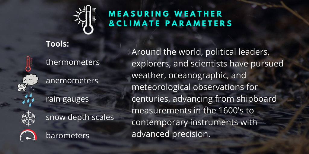
How do we measure climate and weather parameters?
Individual efforts to observe weather in North America began in the mid-17th century, and there were groups of volunteer observers in the U.S.A. since 1776. The U.S. Surgeon General James Tilton ordered Army posts across the U.S.A. in 1814 to begin meteorological observations, giving rise to the first observing network in North America, which was formalized by the Smithsonian Institution in 1849 and the National Weather Service was established in 1870. In Europe, Fernando II de Medici – the Grand Duke of Tuscany from 1621 to 1670 – established a meteorological observations network in ten cities, among them Florence, the home of the Medicis; the collected data were sent to Florence at regular intervals. A few stations in Central England have measured surface air temperature since 1659, but the more reliable record is since 1772. In 1854, the U.K. Government established the U.K. Meteorological Office. The British East India Company established several meteorological observatories in India beginning in 1785, followed by other observatories in the first half of the 19th century. The India Meteorological Department was established in 1875 as a branch of the colonial government. Then, in late 19th and early 20th centuries, national meteorological services were established in many countries in Europe and Asia, although meteorological measurements were started in some countries much earlier. Therefore, reliable instrument-measured observations of precipitation and temperature are available in many countries for well over 100 years.
The recorded history of oceanographic observations goes back to at least the 15th century and Christopher Columbus had also observed a hurricane in the Atlantic. There are other records of shipboard measurements of various oceanographic phenomena and of meteorological phenomena observed at sea. The Challenger expedition in 1872-76 was probably the first, organized, around-the-world cruise that made extensive oceanographic observations. Regular measurements of sea-surface temperatures (SSTs), however, did not begin till the 1850s. In the beginning, most SST observations were made at regular times along shipping routes from Europe to Africa, Asia, and North America. Geographical coverage even in these regions was generally sparse and uneven. The two World Wars in the 20th century interrupted regular measurements; and the opening of the Suez (1869) and Panama (1914) Canals permanently changed shipping routes and, therefore, geographical coverage of oceanographic measurements. In the Pacific Ocean, sparsity of shipping routes and the World Wars made possible regular observations only after the 1940s. Changes in SST measurement instruments and methods also complicated quantitative use of the available data. Some scientists have invested substantial efforts in adjusting land surface air temperature and SST data to correct for biases and changes in measurement techniques.
The vast majority of these measurements have been made with thermometers (temperatures), anemometers (winds), rain gauges (rain), snow depth scales (snow), and barometers (air pressure). Since the advent of Earth-orbiting satellites, temperatures and winds at various heights in the atmosphere, rain and snow, water vapor, atmospheric constituents, vegetation cover, and other parameters have been estimated with remote sensing instruments also. These instruments measure visible and infrared radiations reflected or emitted by the Earth and the atmosphere. Using known physics of how these radiations interact with various atmospheric constituents, temperatures and other parameters are then estimated from the radiation measurements. Ground-based and satellite-based radars are also used to remotely estimate liquid and solid precipitations. Regardless of whether a measuring instrument senses a parameter with physical contact or remotely, a very substantial and careful effort is made to calibrate the instrument against precise sources of parameters, and then a calibrated instrument’s measurements are validated by independent measurements not used in the calibration process. Thus, the measurement of weather and climate parameters involves hundreds of thousands of people around the world every day whose main job it is to make these measurements and provide them for weather and climate analyses and predictions.
How do we study climate variability?
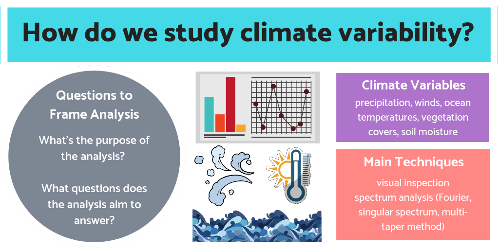
Two main climate variables or parameters of interest to lay people are precipitation (rain, snow, or other forms) and temperature. Climate scientists are also interested in studying patterns of variations in time series of other parameters such as winds, ocean temperatures, snow and vegetation covers, and soil moisture. Many techniques developed for data analysis in other fields have been applied or adapted to climate variability analysis. This is an overview of some frequently used techniques.
Before we begin any analysis, it is very important to decide why we want to do it. Also, we should judge whether the available data are suitable for the purpose(s) we have in mind. If possible, it helps to frame questions we want to address to the data. The selection of technique(s) and interpretation of results depend on the questions. It can be very instructive to inspect a time series visually before putting it through rigorous analysis. A visual inspection can tell us if there is a linear trend (increasing or decreasing) in the time series, if there are prominent cycles in the time series, and if there are discontinuities in the time series. If there is a linear trend from the beginning to the end of the time series, the slope and intercept of the trend should be estimated and the trend should be removed from the time series before applying any analysis technique. Then, if one of the questions we framed is “Are there prominent cycles and what are their periods?”, we should apply some type of spectrum analysis technique which shows strengths of cycles (or oscillations) as a function of cycle period. Each technique has positive and negative aspects which must guide the selection and later interpretation of results. Some commonly used techniques are Fourier, Singular Spectrum, and Multi-Taper Method. Results from these techniques can be plotted as a graph of oscillation frequency (or period) on the x-axis and the strength of each oscillation on the y-axis. Results from each of these techniques should be compared with chance occurrence of prominent cycles; such comparisons are known as assessment of statistical significance of results. Results can also be checked qualitatively against “poor man’s spectrum analysis” in which the total length of a time series is divided by the number of prominent peaks (or valleys) in the time series. This ratio gives an estimate of the most prominent cycle period in the time series. In an extension of spectrum analysis techniques known as filtering, unwanted cycle periods (or oscillation frequencies) can be removed and only the remaining components of a time series can be examined. For example, if we want to study only the climate variability with cycle periods longer than 10 years, we can filter out shorter periods and only the variability longer than 10 years can be studied.
If there are two time series of equal lengths and if we want to see if the two are statistically related, we can estimate the correlation coefficient between them. This coefficient can be calculated for simultaneous correlation and also for time delays (known as lags) between the two series by sliding one series with respect to the other. For example, suppose we want to know if rain at two locations 100 km apart is related to each other, we can estimate lagged correlation coefficients between the two rain time series. If the storm causing the rain in both locations is moving from west to east, the western location will experience rain first and then the eastern location will experience it after some time. The lagged coefficients may show this time delay. As in most statistical analysis techniques, it is very important to compare correlation coefficient results with an assessment of chance occurrence to ascertain reality of the correlation.
Extending the previous example further, let’s say that there are more than two time series on an x-y grid, with a time series at each node of the grid. So, now we have 3-dimensional data to analyze. If we want to know if there are dominant patterns in these data, we can apply an extended version of the correlation coefficient analysis. We can select one reference point in the x-y grid and estimate correlation coefficient between the reference point and all grid points. This will give us a map of correlation coefficients which may indicate if there is a large-scale pattern extending around the reference grid point. Such correlation maps can be constructed for several reference points to see if there are dominant patterns in the data. In a more advance technique known as the Empirical Orthogonal Function or Principal Component analysis, a matrix made up of such correlation coefficients can be analyzed to identify dominant patterns defined by their strengths (or variances) and the time evolution of each pattern can also be calculated.
What are weather and climate models and how they are used?
Air and water are fluids. Therefore, motions and temperatures of atmosphere and ocean are governed by principles of fluid dynamics and thermodynamics. These principles are formulated in terms of mathematics. Since the motions and temperatures are functions of several variables such as space (longitude, latitude) and time, the so-called laws of motion and temperature are express time and space evolutions of winds, ocean currents, and temperatures as differential equations. These equations also incorporate laws of thermodynamics because air and water absorb as well as give up heat. Other differential equations govern evolutions of water vapor, chemical constituents, and salt in the oceans. Since water can exist in air as solid, liquid, or vapor depending on air temperature, processes which convert any of these phases to other phases are also included in the governing equation for water vapor as are processes of evaporation and precipitation (rain, snow, or other forms of precipitation). Processes which form clouds, which dissipate momentum by friction, which transfer heat, and which change salt content of ocean water are also included in the governing equations. Finally, an equation describing expansion/contraction of air or water column is also included in the governing equations.
These equations contain non-linear terms, derivatives with respect to time and space co-ordinates, and localized heat-momentum-water transfer processes, so they cannot be solved analytically and have to be solved numerically. There are various numerical methods of solving these equations, but the simplest method is to define a longitude-latitude-height grid centered on the geographical area of interest and to “solve” the governing equations at each grid point by approximating derivative terms as finite differences. Numerical methods have been developed which conserve momentum, heat, and other physical quantities as required by the principles of fluid dynamics and thermodynamics. The last requirement is to define motion, temperature, salt, water vapor, etc. conditions at the boundaries of the grid domain. These governing equations are then solved with powerful computers. The finer the grid spacing, the larger the computing power needed to solve the governing equations.
For short term weather forecasting, only the atmosphere model is used and boundary conditions such as land and snow cover, and ocean temperature are kept fixed; these are usually based on observed data for the region of interest. For long term climate simulation and forecasting, an atmosphere model is coupled to ocean and land models such that variables of these models interact in space and time, and boundary conditions are fixed for the entire atmosphere-ocean-land system being modeled. Besides climate simulation and forecasting, such coupled climate models are also used in estimating potential impacts of changes in land cover-land use, urbanization, desertification, forestation/de-forestation, and changes in atmospheric constituents such as CO2, methane, and volcanic material. Potential effects of changes in incoming solar radiation are also estimated with coupled climate models. Such models require much more computing power compared to short term weather forecasting models.